Session 2 Tutorial:
Introduction to the Ceres High-Performance Computing System Environment
This page contains all the info you need to participate in Session 2 of the SCINet Geospatial Workshop 2020.
Zoom session recording (USDA eAuth required), Zoom session chat
Learning Goals:
- understand what an HPC system is and when to use one
- introduction to the USDA-ARS Ceres HPC system on SCINet
- access the Ceres with Secure Shell at the command line and with the JupyterHub web interface
- create a simple Jupyter notebook
- execute basic linux commands
- run an interactive computing session on Ceres
- write and run a SLURM batch script on Ceres
Contents
High-Performance Computing (HPC) System Basics
Ceres HPC Login with Secure Shell (SSH)
Ceres HPC Login with JupyterHub
Interactive Computing vs Batch Computing
Submitting a Compute Job with a SLURM Batch Script
Session Rules
GREEN LIGHT, RED LIGHT - Use the Zoom participant feedback indicators to show us if you are following along successfully as well as when you need help. To access participant feed back, click on the “Participants” icon to open the participants pane/window. Click the green “yes” to indicate that you are following along successfully, click the red “no” to indicate when you need help. Ideally, you will have either the red or green indicator displayed for yourself throughout the entire tutorial. We will pause every so often to work through solutions for participants displaying a red light.
CHAT QUESTIONS/COMMENTS TAKE FIRST PRIORITY - Chat your questions/comments either to everyone (preferred) or to the chat moderator (Rowan or Kerrie - whoever is not actively presenting) privately to have your question/comment read out loud anonamously. We will address chat questions/comments first and call on people who have written in the chat before we take questions from raised hands.
SHARE YOUR VIDEO WHEN SPEAKING - If your internet plan/connectivity allows, please share your video when speaking.
KEEP YOURSELF ON MUTE - Please mute yourself unless you are called on.
The SCINet Website
The SCINet Website is the source of much of the material presented in this tutorial. Use the SCINet website to request SCINet accounts, access SCINet/HPC user guides, get computing help or other support, and find out about upcoming and previous computational training events.
High-Performance Computing (HPC) System Basics
What is an HPC System?
A High Performance Computing (HPC) system provides a computational environment that can processes data and perform complex computations at high speeds. Generally HPC systems consists of 3 components:
-
Compute nodes (servers) that can provide a consistent environment across the system (similiar OS, software, etc…).
-
Data storage, generally a parallel file system, that supports high I/O throughput.
-
Highspeed network to allow for effecient communication and data transfer across compute nodes.
For specific details about the Ceres system see: https://scinet.usda.gov/guide/ceres/#technical-overview
Why use an HPC System?
HPC systems can provide the compute infrastructure that allow researchers to improve or make possible computationally intensive analyses/workflows. However, developing analyses to run on HPC systems involve a non-trivial amount of overhead. Therefore, you should first evaluate if SCINet is an appropriate avenue for your research. Typically, analyses that are well-suited for SCINet are:
- CPU intensive workloads
- high memory workloads
Additional considerations are:
- Are my analyses already optimized?
- Will I need to parallelize my analyses (typical for CPU intensive workloads)?
- Will I require more than a single node of compute power (ie. distributed computing)?
HPC Terminology
SSH - Secure Shell is a network protocol that allows remote access over un-secure networks. We will use SSH to access the Ceres login node.
shell - a shell is what provides you an interface to the unix operating system. It’s where we type commands and run programs. The default shell on Ceres is called bash.
login/compute node - Nodes refer to the individual servers that compose an HPC system. The login node is the node/server that users are sent to when they SSH to the system. The compute nodes (typically the bulk of the HPC nodes) are designed for running the computationally intensive workloads. There can be many different types of compute nodes within a HPC system (i.e. standard, high memory, gpu, etc…).
core/logical core - Cores (or CPU) are the computational processing component within a computer. Most modern cores have hyperthreading, which allow a single core to process two tasks simultaneously. Therefore, logical cores refer to the number apparent (not physical) cores in a system. For most modern systems, a single core will equate to two logical cores.
batch/interactive computing - Batch computing referes to workflows that require no user interaction once they are underway/submitted. Interactive computing typically involves processing commands/transactions one at a time and requires input from the user.
SLURM/job scheduler - HPC systems generally have software to allocate resources (nodes, cores, memory, etc…) in a fair and consistent manner to the users. These systems are generally refered to as job schedulers. A common job scheduling software used in HPC systems is SLURM.
USDA-ARS HPC System Details
The Computer Systems page of the SCINet website gives a brief summary of the USDA-ARS HPC systems.
The Ceres HPC System
The Ceres User Manual and Ceres Quick Start Guide contain most of the information you could want to know about the Ceres HPC.
System Configuration
The operating system running on Ceres is CentOS and the job scheduler is SLURM. See System Configuration in the Ceres User Manual for more.
Nodes
When you SSH into Ceres you are connecting to the login node. The login node should be used for navigating your directories, organizing your files, and running very minor scripts. All computing on Ceres should be done on compute nodes. DON’T RUN YOUR COMPUTE SCRIPTS OR INSTALL SOFTWARE ON THE LOGIN NODE AS IT SLOWS THE NODE DOWN FOR EVERYONE.
When you use JupyterHub to login to Ceres you are placed on a compute node, not a login node.
There are 5000+ compute cores (10000 logical cores), 65 TB of total RAM, 250TB of total local storage, and 4.7 PB of shared storage available on the Ceres HPC. See the Technical Overview in the Ceres User Manual for more.
Partitions/Queues
All Ceres users have access to the “community partitions”- short, medium, long, long60, mem, longmem, mem768, debug. Each different partition has different capabilities (e.g. regular memory versus high memory nodes) and resource restrictions (e.g. time limits on jobs). The short partition is the default. See Partitions or Queues in the Ceres User Manual for more.
Some research groups have purchased their own nodes which are placed on “priority partitions” that the research group has first priority to use. Other Ceres users have lower priority access to many of these partitions (the “-low” and “scavenger” partitions). However, the “-low” partitions have a compute time limit of 2 hours and while you can run jobs for much longer on the “scavenger” partitions, you run the risk of having your job killed at any moment if a higher priority user needs access to the nodes.
Directory structure and data storage
There are 3 places to store your codes and data persistently on Ceres:
- home directory, /home/firstname.lastname/ - Everyone has a small private home directory. You are automatically put in this directory when you log in. Home directories are backed up. You shouldn’t run computations from your home directory.
- project directory, /lustre/project/your_project_name/ - You must apply for each project directory. This is where you run scripts from and where your datasets, codes, and results should live. Project directories are not backed up.
- keep directory, /KEEP/your_project_name/ - Each of your projects will also have folder in the /KEEP directory. This folder is backed up nightly. Copy your most important project files to your /KEEP folder to ensure they are backed up. Compute jobs shouldn’t be run from /KEEP directories.
Temporarily share files locally with other users:
- project shared files directory, /lustre/project/shared_files/ - Everyone has access to the shared files folder in the project directory. You can share files with other users by creating a folder inside this directory a copying your files there, although there is a 5GB limit. This is not a permanent storage location for your files.
See more about directories and data storage in Data Storage in the Quick Start Guide and in Quotas in Home and Project Directories in the Ceres User Manual.
User Compute Limitations
There is currently no quota system for keeping track of how many jobs you run or how much compute time you’ve used on Ceres like there is on University and National Lab HPC systems. However, there is a fair share policy which means super users who run many jobs and take up a lot of compute time are downgraded in priority compared to other users.
The individual user compute limitations are:
- 400 cores per user (across all your running jobs)
- 1512 GB memory per user (across all your running jobs)
- 100 jobs per user running simultaneously
Software on Ceres
There is plenty of software on Ceres that you can access through the module system. See the Software Overview for more.
Users can also install their own software using the Anaconda package and environment management software module. See the Conda Guide from more.
If you don’t want to use Conda, Ceres is also set up for R and Perl users to download packages. See the Guide to Installing R, Perl, and Python Packages for more (although we recommend that Python coders use Conda).
Lastly, if none of the above methods of accessing software work for your particular software needs, you can request that the SCINet Virtual Research Support Core install software on the system for you. This is the method of last resort though because it takes a few weeks and requires an agency-level security review. See the Request Software page for more.
Getting data on/off
There are multiple ways of getting data on and off of the Ceres HPC system. See the SCINet File Transfer Guide for more.
- for data on the web, download directly to Ceres using tools like wget
- for data on your local machine the recommended method is Globus
- for large local data, you can:
- utilize the I2 connection at your ARS location or
- ship to VRSC and they will upload for you
User support from the Virtual Research Support Core (VRSC)
The VRSC is comprised of Iowa State University and ARS staff who manage the Ceres HPC system and provide support to users. See more on the SCINet VRSC Support page.
Ceres HPC Best Practices
- nothing serious should be run on the login node
- run compute jobs from project directories
- install software on a compute node (salloc)
- install software (including Conda environments) in your home or /KEEP directories
- use node local scratch space for faster i/o with large datasets (stage your data to /local/scratch, $TMPDIR)
- use your /KEEP directory to ensure important data/codes are backed up
- for short heavy compute jobs (less than 2hrs) go for the brief-low partition (more cores per node and more memory)
- acknowledge SCINet in your pubs!
Other SCINet HPC Systems
There are two other HPC Systems coming to SCINet soon. Summaries of the systems will be posted to the SCINet website computing systems page.
Ceres HPC Login with Secure Shell (SSH)
First, let’s login to our SCINet (Ceres) accounts with SSH. You should have already successfully logged in this way at least once before today by following the instructions sent to you when your SCINet account was approved. The Quick Start Guide has instructions for SSH’ing to Ceres from Windows, Mac, and Linux Machines.
If you haven’t yet set up a config file for SSH’ing to Ceres (we won’t cover it but instructions are at the Quick Start Guide link above) then:
ssh -o TCPKeepAlive=yes -o ServerAliveInterval=20 -o ServerAliveCountMax=30 firstname.lastname@ceres.scinet.usda.gov
The keep alives are especially important for rural/satellite internet connections so that instantaneous breaks in service won’t terminate your connection to the HPC.
If you’ve set up your config file you can simply:
ssh whatever-you-named-the-host-in-your-config
If you are not on an ARS VPN, you will be asked for a 6-digit Google Authenticator code. See the multi-factor authentication guide for help. After entering the Google code, you will be asked to enter your password.
If you are on an ARS VPN, you will skip the Google authentication and be asked only for your password.
After a successful login you will see a list of all your quotas and used space.
If you can’t successfully login to your account, contact scinet_vrsc@usda.gov for assistance.
To sign out of Ceres just close your terminal or type exit.
Ceres HPC Login with JupyterHub
In summer 2020, a new way of accessing Ceres was set up with JupyterHub. JupyterHub allows access to Ceres through a web browser and spawns an instance of JupyterLab on a compute node.
Let’s walk through how to login to Ceres using JupyterHub with the Jupyter Guide.
Tour of JupyterLab
The Launcher: Click the plus sign on the left or go to File > New Launcher to see the launcher screen. From here you can open a Jupyter Notebook, a terminal, a textfile, a markdown file, and more.
Accessing your files: Clicking on the folder icon on the far left will show you the files and folders in your home directory or the directory you listed in the JupyterLab spawner during the login process.
Access to software modules:
Clicking on the hexagon icon on the far left will show you all the software modules available on the Ceres HPC. Clicking load on any of the modules is equivalent to typing module load name-of-software (as described in the Quick Start Guide). Note: there aren’t a ton of software modules on Ceres that are relevant to the geospatial research community, so you likely won’t need to use this feature often.
Jupyter Notebook Basics
Step 1: Open a Jupyter Notebook
Click the launcher and launch a Python 3 notebook- notice the .ipynb file extension.
Notice how it says “Python 3” at the top right of the notebook. You are working in a Python 3 environment or “kernel”. You could change this by clicking on “Python 3” and selecting a different kernel from the dropdown list in the pop-up box. Don’t choose a different kernel for now, but note that this is where you could select a Conda environment that you have created. We will cover this in the Session 4 Tutorial on computational reproducibility.
Step 2: Add a Raw Text Cell
At the top of the notebook click “Code” and change it to “Raw”. Click on the cell and type the following:
author: your name
date: today's date
description: my first jupyter notebook hello world
To execute the cell type Shift+Enter or click the run button at the top of the notebook (looks like “play”).
Step 3: Add a Markdown Cell
Click inside the new cell that has appeared in your notebook, then at the top of the notebook click again on “Code” and change it to “Markdown”. Click inside the Markdown cell and type:
# Make Notes in Your Codes Prettier Using Markdown
## add a subtitle

Write some pretty text.
Execute the Markdown cell.
Learn more about JupyterHub markdown syntax here or here. A quick Google search on “JupyterHub markdown cheat sheet” will reveal tons of helpful sites.
Step 4: Add a Code Cell
If you executed the previous cell, a new code cell should have automagically appeared. Type:
print('Hello, Jupyter world!')
and execute the cell.
Notice how the output appears right in the Jupyter notebook. You can also print tables and plot figures right in the Jupyter notebook… all your code, comments, and outputs will be in one place- inside the .ipynb file!
Step 5: Delete a Cell
Right click on the cell and choose “Delete Cells” or place your cursor in the cell and then click on the scissors icon at the top of the notebook.
Step 6: Insert a Cell
Insert a cell under the markdown cell by clicking on the markdown cell and then clicking the plus button at the top of the notebook (next to the scissors). Type:
print('How awesome is this?!')
and execute the cell.
Step 7: Clear all Outputs
At the top of JupyterLab click Kernel > Restart Kernel and Clear All Outputs, the click Restart in the pop-up window. All you outputs are now cleared.
Step 8: Re-run all Cells
At the top of JupyterLab click Run > Run All Cells
Step 9: Save Your Work
Actually, JupyterLab is autosaving your notebook as you work, but you’ll want to name your file.
Right click on “Untitled.ipynb” either on the notebook tab or in the file browser on the left, then choose “Rename”. In the pop-up window, name your file and click “Rename”.
Basic Linux Commands
Now we’ll work through some basic linux commands. For more commands than we cover here see the Unix Basics Tutorial from the bioinformatics workbook created by Andrew Severin of Iowa State University/SCINet VRSC.
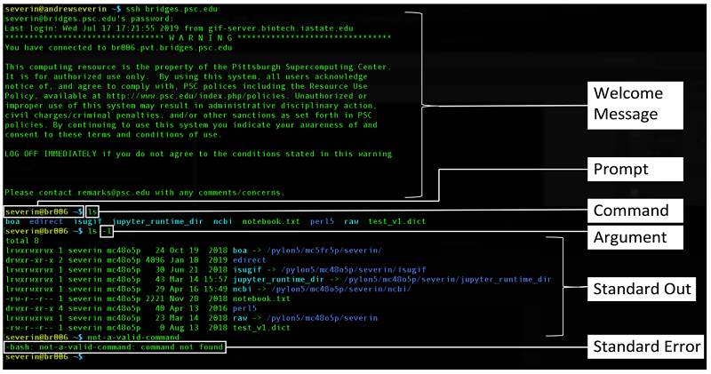
First an illustration of the following terms:
- prompt,
- command,
- argument (a.k.a options, flags),
- standard out (stdout),
- standard error (stderr)
What directory am I in?
pwd - print the path of the working directory (the directory that you are current in) to the screen (standard out)
pwd
stdout should show /home/firstname.lastname. This directory can be accessed with ~, $HOME, or by typing only cd (all of which we will cover later).
How to make a new directory (folder)
mkdir - make a new directory
mkdir mynewdirectory
You have now created a new empty directory inside of your home directory. To see it we will use ls
How to list (see) files and directories
ls - list directory contents
ls
You should see your new directory along with other files and directories that you have in your home directory.
To view all files and directories (including hidden ones that start with a “.”) add an option/flag to the ls command:
ls -a
you will get the same result with:
ls --all
Note that many options are accessible using the long version which always starts with two dashes (–all) or using the abbreviated version which always starts with one dash (-a).
Also, you can add multiple options to commands:
ls -alh
will show you all files in your working directory in the long listing format (-l) and with file sizes listed in human-readable format (-h). The -l option shows you permissions, ownership, size, and last-modified date.
Here’s a key to the long format ls -l:
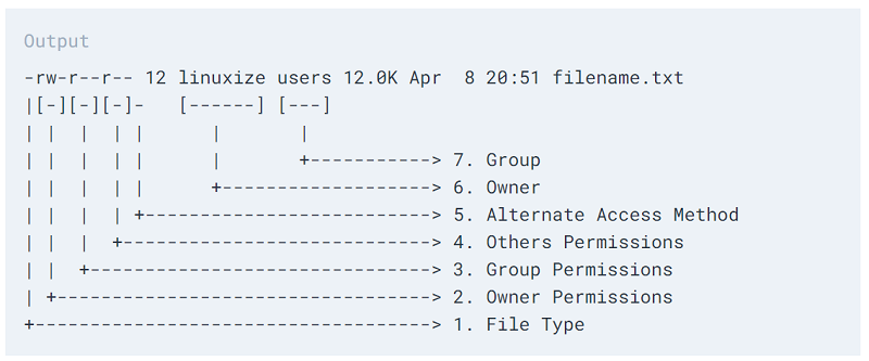
We’ll come back to how to change file or directory permissions.
What options are available for each command?
man - to view the reference manual for a command which will show the command format and all the available options.
man ls
So many options! Don’t worry, you don’t have to know all the options for every command. To view the entire manual page, use your up/down arrows to scroll or your pg up/pg dn buttons.
NOTE: If you haven’t discovered it already, YOUR MOUSE DOESN’T WORK AT THE COMMAND LINE! Notice the -a, -l, and -h on the man page for the ls command.
To exit/quit the man page:
q
Change Directory
cd - change directory
Move from your home directory into your new directory with:
cd mynewdirectory
Look at what directory you are in now:
pwd
You should be at /home/firstname.lastname/mynewdirectory
To go up/back directory levels use “..”:
cd ../..
takes you back two levels to the /home directory, where if you ls you will see the home directories all of users.
Go back to mynewdirectory with:
cd ~/mynewdirectory
Note how the “~” is a shortcut for /home/firstname.lastname. Another shortcut for your home directory is $HOME. Replacing ~ with $HOME in the above command would yield the exact same result.
To get back to your home directory from anywhere, just type cd with no arguments:
cd
Creating a text file with nano
nano - a terminal-based text editor. This means when you use nano, your prompt will dissapear and you will instead be editing a text file on your terminal screen. There are plenty of other terminal-based text editors but we won’t cover them here.
First, change directory into mynewdirectory.
Then, open a new empty text file:
nano
You can recognize that you are now in the nano text editor due to the banners on the top and bottom of your terminal. The top banner will say the nano version, the bottom banner shows shortcut keys to help you use the editor.
Let’s write in our new text file:
1
dog
then type Ctl+x, then y to save, the type the name file1.txt and hit enter.
See that you made a file called file1.txt with:
ls
Let’s do it again. This time we’ll create a file with a name right off the bat:
nano file2.txt
Inside nano type:
2
Dogs
then Ctl+x, y, enter. You should now be back at your command prompt.
Let’s create one more text file that we’ll do more things with in a minute. Use nano to create file3.txt and type the numbers 1-15 on separate lines in the text file, then save the file.
Viewing the contents of a text file
head - print the first 10 lines of the file to stdout
tail - print the last 10 lines of the file to stdout
cat - concatenate and print all contents to stdout
Let’s try these out:
head file3.txt
tail file3.txt
cat file3.txt
cat file1.txt file2.txt file3.txt
The last command should concatenate the printing of all three files to stdout.
Using cat to create textfiles
cat - concatenate and print all contents to stdout.
You can actually use cat to create quick textfiles without using nano.
cat > file30.txt
After you issue this command you’ll see your cursor move to the next line in the terminal. Type whatever you want, multiple lines if you want. Cat will put whatever you type into a file called file30.txt. When you are finished typing you must type Ctl+d at least once to execute the command.
An ls should now show that you’ve created file1.txt, file2.txt, file3.txt, and file30.txt
Wildcards
* - matches at least one character
? - matches a single character
[] - matches the characters inside the brackets
To better understand how to use wildcards we’ll practice with ls:
List all files that start with “file” and end with “.txt”:
ls file*.txt
List all the files that start with “file”, have one character after that, and end with “.txt”
ls file?.txt
Notice how this did not list file30.txt because the ? matched only a single character. You can however use two single character wildcards in a row:
ls file??.txt
should list only your file30.txt
Let’s get fancier now by using the brackets:
ls file[1-3].txt
and you will get the same result with
ls file[1-3].*
which should list only file1.txt, file2.txt, and file3.txt
What do you think the following will list?
ls file[1,3].txt
You should see only file1 and file3.
How about this?
ls file[1,3]*
This command will list all files that start with “file” and have a 1 or a 3 somewhere in the filename.
Copying and moving files
cp - copy files and directories
mv - move or rename files
Make a copy of one of your text files:
cp file1.txt file1a.txt
Now list your files to see the new file you created and then view the contents of your new file with the head command.
Let’s make a copy of one of your files to a different directory:
cp file1.txt ../file1.txt
You should now have a copy of file1 one level back in your home directory.
From your mynewdirectory, list the files in your home directory:
ls ~
You should see the copy of file1.txt in your home directory.
Let’s move file2 into your home directory:
mv file2.txt ~
List the files in your home directory to see that file2 was moved.
Let’s move file2.txt from your home directory back into your mynewdirectory:
mv ../file2.txt .
Note how the double dot indicates that the file is located one directory up and the single dot indicates the current working directory.
Let’s rename file2:
mv file2.txt file100.txt
List the files in your working directory to see that you’ve renamed the file.
search files for a word/phrase (“pattern”)
grep - print lines of files that match a pattern
Let’s search our files in the mynewdirectory for the word “dog”:
grep 'dog' *
You should see that two of your files contain the word “dog”. But wait, only two?
grep -i 'dog' *
The -i flag means “ignore case” and will find ‘dog’ a third time. Notice how the word in the file is “Dogs” but grep found it anyway.
To search on an exact word:
grep -i -w 'dogs' *
removing files and directories
rm - remove files or directories
NOTE: there is no “undo” in linux. Be very careful when using the rm command. When you delete something, it’s gone- there’s no trashcan to recover from.
Delete one of your files with:
rm file100.txt
List your files to see that file100 is gone.
Let’s remove a directory next. First make a new directory and move one of your files there:
mkdir delete-me
mv file1.txt delete-me
Try to remove the delete-me directory with the rm command:
rm delete-me
You should get an error. Overcome that error with:
rm -r delete-me
The directory delete-me should now be gone. What’s the -r option mean?
man rm
We can see on the man page for rm that -r means remove directories and their contents recursively.
change file permissions
chmod - change file “mode”
If want to change who has access to certain files and directories, we use chmod (remember though that your home directory is private by default). View the permissions on your files with:
ls -l
You should see that the file owner, and group members can read read and write to these files, but everyone else (“others”) only has read privileges. To add write privileges for everyone else:
chmod o+w file3.txt
ls -l
Now let’s take away all privileges for “others”:
chmod o-rw file3.txt
ls -l
see how much storage you are using
du - estimate file space usage
my_quotas - see a summary of your storage quotas and how much of the quotas you’ve used. only works from your home directory
In your mynewdirectory:
du -h
To list the size of each directory inside your home directory:
cd
du -h --max-depth=1
The max depth flag is often very helpful, otherwise you will get the size of every single file in every single directory.
To see a summary of your storage quotas and how much space you’ve used from each quota, go to your home directory and type:
my_quotas
This is the exact same info that appears when you SSH to Ceres. Note that this command only works from your home directory.
download files/data to Ceres from the web
wget - for downloading files from the web. It’s non-interactive which means you can start something downloading with wget, log off the system before the download finishes, and the download will still be running. wget is not the only way to grab files from the web, but it’s the only one we’ll cover
Let’s get one of my favorite gridded surface air temperature datasets from Berkeley Earth at http://berkeleyearth.org/data-new/. It’s the global monthly land + ocean data on a 1-degree grid.
salloc
wget http://berkeleyearth.lbl.gov/auto/Global/Gridded/Land_and_Ocean_LatLong1.nc
exit
ls -lh
We just downloaded a 407MB data file in a few seconds. Wow, that was easy! More on salloc in a minute…
view metadata of a netcdf file
ncdump - converts netcdf file metadata to text form on stdout
just a quick side note on working with the data file we downloaded…
ncdump -h Land_and_Ocean_LatLong1.nc
This shows metadata on all the data variables that are in the files including dimension information for each data variable (lat, lon, time). There is also metadata about the file history.
Note: the -h flag means “header”, without it you will get thousands of data values printed to stdout. If you do this by accident on a large file Ctl+c will stop the printing to stdout.
View the values of a single data variable with:
ncdump -v latitude Land_and_Ocean_LatLong1.nc
NetCDF is one of my favorite data formats because the spatial and temporal metadata is already “attached” to the data variables in the file. This means that when you go to plot ‘temperature’ from this netcdf file (using python, r, etc) the data will appear automagically on a map without you having to define the longitudes and latitudes.
Let’s all delete this data file so that it’s not sitting on Ceres in 50 different user accounts taking up space. Plus, it’s easy to download again if we ever wanted to.
rm Land_and_Ocean_LatLong1.nc
loading software from the module system
view available software on Ceres with:
module avail
load software (in this case conda) from the module system:
module load miniconda
see what software modules you have loaded with:
module list
unload software from the module system with:
module unload miniconda
There are also some SLURM-specific commands that are very useful
See the bioinformatics workbook for more than what we cover here.
sinfo - see the status of all the nodes
salloc - “SLURM allocate”. Move onto a compute node in an interactive session. More in the next section.
squeue - view information on compute jobs that are running. More in the next section.
scancel - terminate a compute job that is running
sbatch - submit a batch script to run a compute job. More in the next section
Interactive Computing vs Batch Computing
Many geospatial researchers spend much of their time writing and debugging new scripts for each project they work on. This differs from other research communities who may be able to re-use a single script frequently for multiple projects or who can use a standard analysis process/workflow on many different input datasets.
A geospatial researcher may write and debug their scripts using small to medium size data until the script is functional and then modify the script to process big data only once. For this reason, geospatial researchers may more often use interactive computing sessions on an HPC.
Interactive Computing on Ceres
Interactive computing essentially means that you are working directly on a compute node as opposed to using the SLURM job scheduler to submit compute jobs in batches. JupyterHub allows us easy access to interactive computing on the Ceres HPC. Just login to Ceres through JupyerHub and start coding in a Jupyter notebook- you will automatically be placed in an interactive compute session.
But let’s learn how to open an interactive computing session from the command line. This is important when you log in with SSH or if you’ve logged in with JupyterHub but want to compute or install software on a different node than where your JupyterLab session is running.
Step 1: Open a terminal on Ceres
Since we are already in JupyterLab, use the launcher to open a terminal. We could also use Windows Powershell or Mac/Linux Terminal to SSH onto the Ceres login node instead.
Step 2: Start an Interactive Compute Session The simplest way to start an interactive session is:
salloc
Issuing this command requests the SLURM job scheduler to allocate you a single hyper-threaded core (2 logical cores) with 6200 MB of allocated memory on one of the compute nodes. The session will last for 2 days, but will timeout after 1.5 hours of inactivity.
View your runnning compute sessions/jobs with:
squeue -u firstname.lastname
To exit the interactive session:
exit
For more control over your interactive session you can use the srun command instead of salloc using the format:
srun --pty -p queuename -t hh:mm:ss -n cores -N nodes /bin/bash -l
srun --pty -p short -t 03:00:00 -n 4 -N 1 /bin/bash -l
will request the SLURM job scheduler to allocate you two hyper-threaded cores (4 logical cores) with 3100x4 MB of allocated memory on one of the compute nodes in the short partition. The session will last for 3 hours, but will also timeout due to inactivity after 1.5 hours.
Batch Computing on Ceres
Batch computing involves writing and executing a batch script that the SLURM job scheduler will manage. This mode of computing is good for “set it and forget it” compute jobs such as running a climate model, executing a single script multiple times in a row, or executing a more complicated but fully functional workflow that you know you don’t have to debug. We’ll cover how to write and execute a batch script next.
Submitting a Compute Job with a SLURM Batch Script
Let’s practice by submitting a batch script.
First create simple python program:
cat > hello-world.py
print('Hello, world!')
then type Ctl-d to exit.
View the file you just created:
cat hello-world.py
a serial job that runs a python script one time
Now create your batch script with nano or other text editor:
nano my-first-batch-script.sbatch
In the nano editor type:
#!/bin/bash
#SBATCH --job-name=HelloWorld
#SBATCH -p short              #name of the partition (queue) you are submitting to
#SBATCH -N 1                  #number of nodes in this job
#SBATCH -n 2                  #number of cores/tasks in this job
#SBATCH -t 00:00:30           #time allocated for this job hours:mins:seconds
#SBATCH -o "stdout.%j.%N"     # standard output, %j adds job number to output file name and %N adds the node name
#SBATCH -e "stderr.%j.%N"     #optional, prints our standard error

module load python_3
echo "you are running python"
python3 --version

python3 hello-world.py
Exit the nano editor with Ctl+O, enter, Ctl+X.
Submit your batch script with:
sbatch my-first-batch-script.sbatch
Check out the output of your compute job. It’s in the stdout file:
ls
cat stdout.######.ceres##-compute-##
Note: there are a ton of other SBATCH options you could add to your script. For example, you could receive an email when your job has completed (see the Ceres User Manual) and lots more (see the SLURM sbatch doc).
Also Note: this is a serial job, meaning that it will run on a single compute core. The compute likely won’t be any faster than if you ran this type of job on your laptop. To run your hello-world code in parallel from a batch script (multiple times simulataneously on different cores) you would use openMP or MPI (see the Ceres User Manual) and your code would have to be in C or Fortran (not Python). For Python coders, there are much easier ways to run in parallel (using interactive mode as opposed to batch scripting), which we will cover in Session 3: Intro to Python and Dask.
a serial job that runs a python script five times
Let’s now run a script that will execute the same python code 5 times in a row back to back.
First, delete all your stdout and stderr files so it’s easier to see which new files have been generated:
rm std*
Now modify your sbatch script using nano to look like this:
#!/bin/bash
#SBATCH --job-name=HelloWorld
#SBATCH -p short              #name of the partition (queue) you are submitting to
#SBATCH -N 1                  #number of nodes in this job
#SBATCH -n 2                  #number of cores/tasks in this job
#SBATCH -t 00:00:30           #time allocated for this job hours:mins:seconds
#SBATCH -o "stdout.%j.%N"     # standard output, %j adds job number to output file name and %N adds the node name
#SBATCH -e "stderr.%j.%N"     #optional, prints our standard error

module load python_3
echo "you are running python"
python3 --version

for i {1..5}
do
  python3 hello-world.py
done
Look at a stdout file and you will see the python code ran 5 times.
Go ahead and delete your stdout and stderr files again.
a parallel job that runs a python script 10 times simultaneously on different cores
Let’s now run a script that will execute the same python code 10 times simulataneously. Modify your sbatch script to look like this:
#!/bin/bash
#SBATCH --job-name=HelloWorld
#SBATCH -p short              #name of the partition (queue) you are submitting to
#SBATCH -N 1                 #number of nodes in this job
#SBATCH -n 10                 #number of cores/tasks in this job
#SBATCH --ntasks-per-core=1
#SBATCH -t 00:00:30           #time allocated for this job hours:mins:seconds
#SBATCH -o "stdout.%j.%N"     # standard output, %j adds job number to output file name and %N adds the node name
#SBATCH -e "stderr.%j.%N"     #optional, prints our standard error
#SBATCH --array=1-10          #job array index values

module load python_3
echo "you are running python"
python3 --version

python3 hello-world.py
You should see a stdout and stderr file for each job in the array of jobs that were run (10) and and the jobs should have run on a variety of different nodes.